Have you ever tried to schedule 1,000 people with different skills, shifts, breaks, and labor rules in a spreadsheet? If you run a large support team, this is a daily reality.
Here is what a schedule looks like for one of our customers:
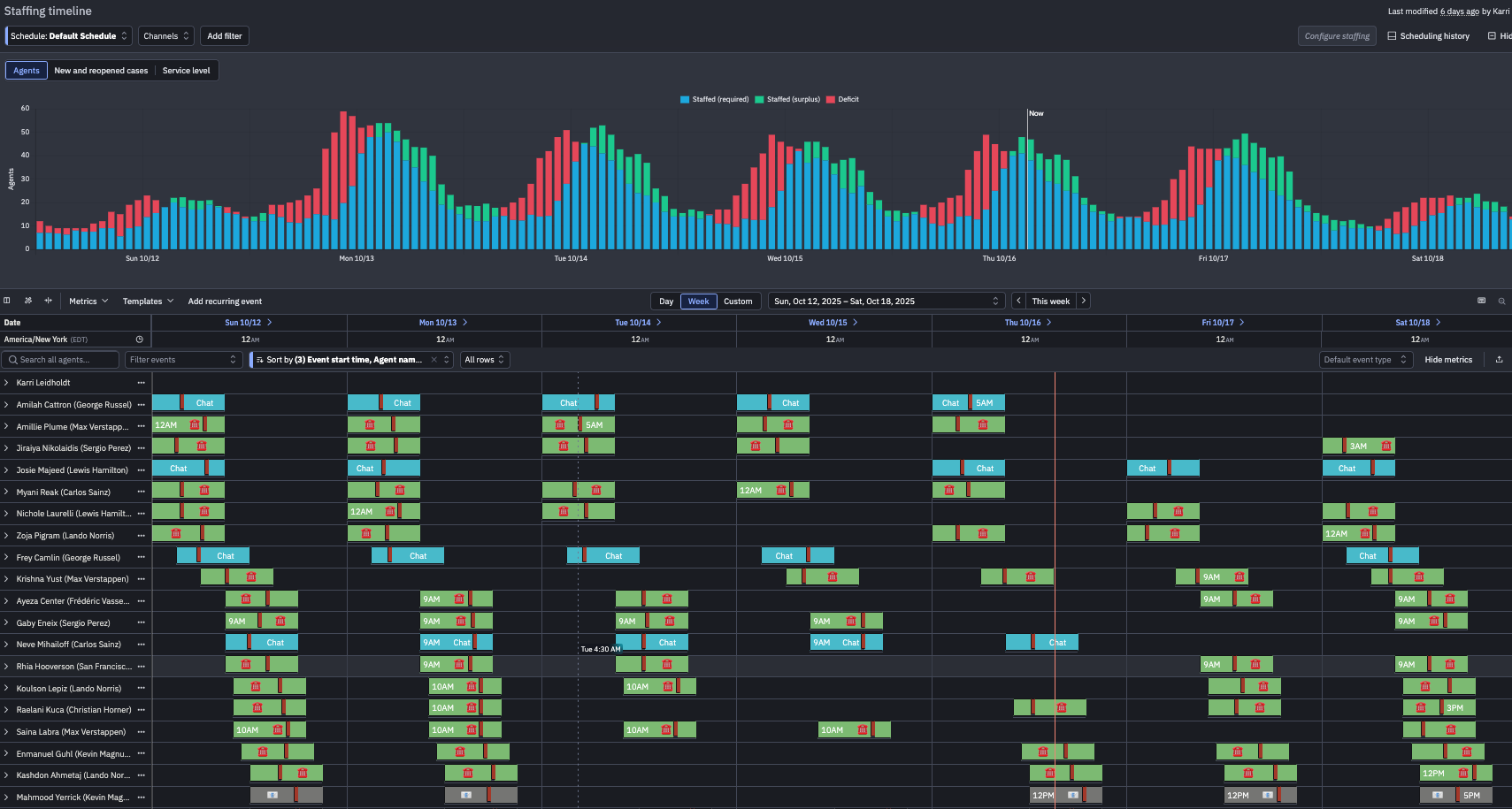
The planner has to follow labor laws like required breaks and max consecutive working hours, respect skills and languages, and match capacity to spiky demand.
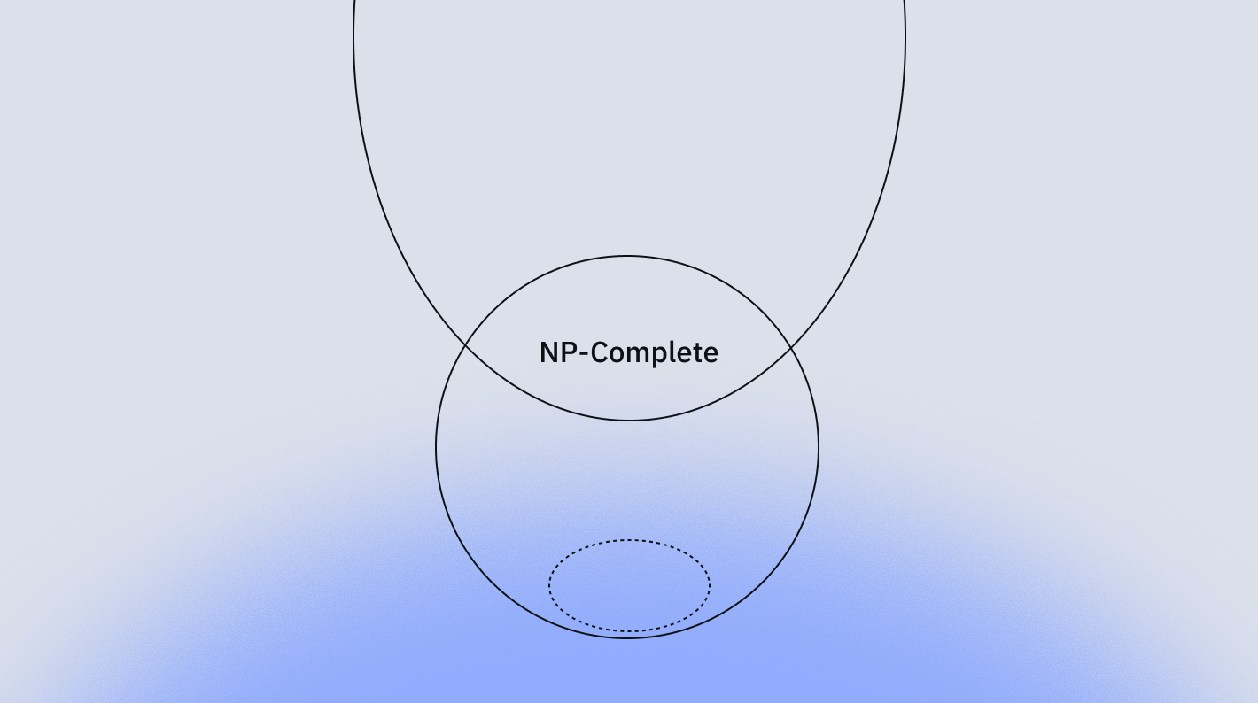
There are around 10³⁰⁰⁰⁰ schedule combinations to consider, and just writing down each digit of this number would take ~15 pages [0]. Because this is an NP-Hard problem, the number of combinations grows exponentially with each additional person being scheduled.
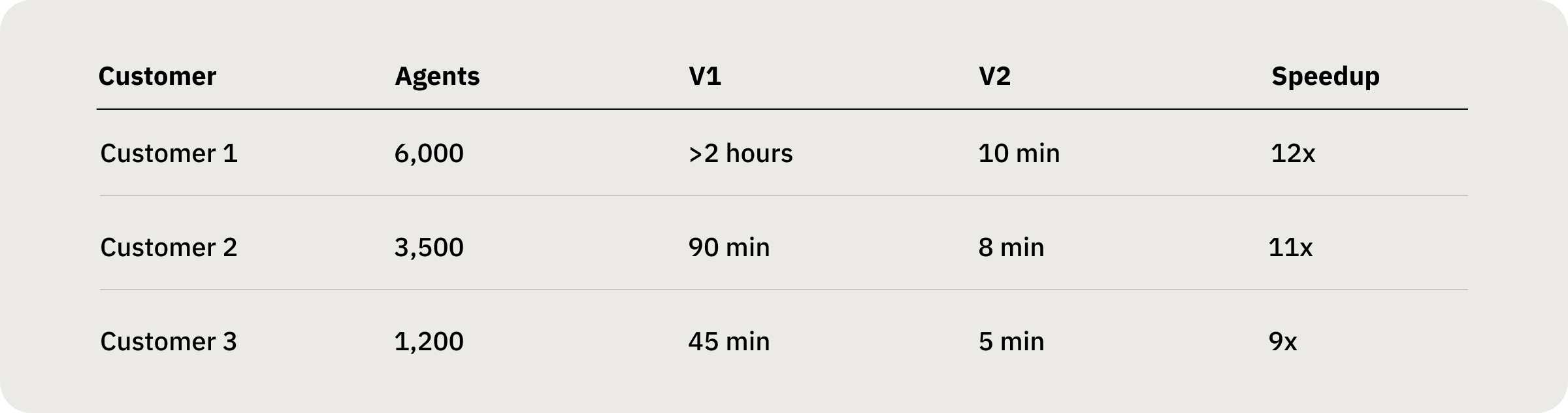
At Assembled, we've built technology to solve this at scale. We schedule tens of thousands of agents for companies like DoorDash, Block, and Stripe, and we've made it 12× faster. This post explains how we turned a 2-hour process into 10 minutes while maintaining schedule quality.
Problem and context
As we began onboarding larger enterprise customers to our schedule generation platform, we stress-tested our system with large-scale datasets. The results were poor: Our monolithic solver that handled 100 agents efficiently would take over 2 hours for a 1,000-agent configuration.
The complexity stems from the interdependencies in workforce scheduling. Each agent brings a unique combination of skills, availability windows, and contractual constraints. They serve different channel/queue combinations with specific service level requirements. In contact centers, channels represent communication methods (chat, phone, email) while queues represent skill-based routing (billing, technical support). Add mandatory breaks, meetings, training sessions, and labor law compliance, and the constraint satisfaction problem becomes computationally intractable at scale.
Our existing approach of feeding all constraints into a single solver instance hit fundamental scalability limits. Solve time exploded as the solver tracked millions of decision variables and their interactions.
Schedule generation algorithm overview
Our algorithm uses a two-step approach, combining the strengths of integer linear programming (ILP) for optimal search and constraint programming (CP) for constraint satisfaction.
- Productive event generation: The primary objective is to maximize coverage of the generated events across all channel and queues. The ILP model uses advanced optimization like cutting planes and column generation to efficiently improve the objective.
- Non-productive event generation: Customers use our rule system to govern valid event placements. A CP model provides a natural framework to encode these rules and a powerful search mechanism to validate large combinatorial spaces.
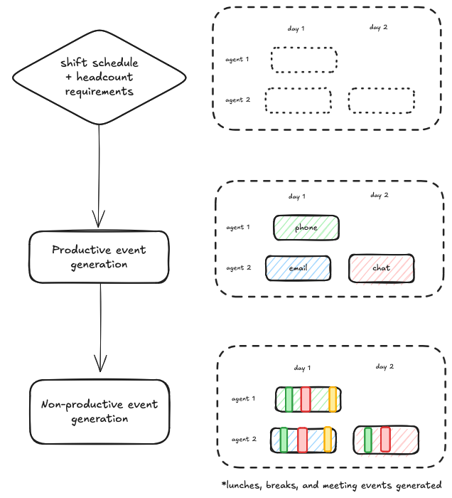
Step 1: Productive event generation (integer linear programming)
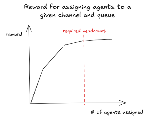
The objective function of our ILP implements a tiered reward system for maximizing coverage:
We use a piecewise linear function to approximate the marginal benefit of covering the headcount requirement for a given time, channel, and queue combination. This incentivizes the solver to spread out agents across channels and queues while still keeping the objective linear.
Step 2: Non-productive event generation (constraint programming)
Using a CP solver, we place mandatory events (breaks, meetings, trainings, etc.) while respecting complex event constraints. Our constraint model supports:
- Interval constraints: Events must occur within specific time windows (e.g., agents must have one lunch, and it must be between the third and fifth hour of their shift).
- Periodic constraints: Events recurring every X hours (e.g., agents must take a break every 3 hours).
- Relational constraints: Events maintaining temporal relationships (e.g., after working the phone for more than 2 hours, an agent must have a 15-minute cooldown event right after).
- Synchronous constraints: Multiple agents sharing events simultaneously (e.g., the entire team must have a meeting once a week when headcount requirements are low).
Problem decomposition: Divide and conquer
Naively using this algorithm at scale is incredibly slow because there are simply too many combinations of scheduling decisions for the algorithm to consider. Our improvement came from recognizing that many shifts don't interact. Agents working different times or serving different channels and queues can be scheduled independently. This insight led to our decomposition strategy:
1. Temporal decomposition
We identify shifts with minimal time overlap:
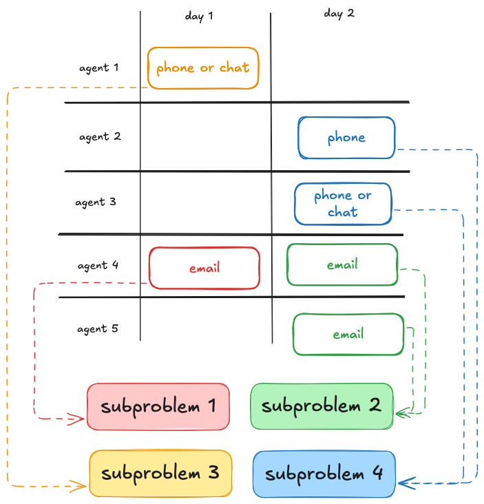
2. Channel queue decomposition
Agents that are eligible for non-overlapping channel/queue combinations can be scheduled independently since their coverage contributions are independent:
Building the decomposition graph
We construct an overlap graph where nodes represent shifts and edges indicate dependencies. Connected components in this graph form our independent subproblems:
This approach decomposed one customer’s 34,000 weekly shifts into 50 independent subproblems, each solvable in parallel. This graph-based formulation turns a global scheduling problem into a set of loosely coupled local problems, reducing solver search space.
Engineering improvements
We use Argo Workflows on Kubernetes to orchestrate the scheduling pipeline. Unlike lightweight async job runners, this setup gives us control over compute resources and first-class support for long-running stateful workflows. Argo also provides observability and retry semantics out-of-the box. The parallelization happens within the container using Python's ProcessPoolExecutor:
1. Parallel processing architecture
2. Dynamic resource allocation
Our pre-processing step analyzes the problem size and requests appropriate memory. Argo dynamically configures the pod resources based on this analysis.
Results: From hours to minutes
Combined with pipeline optimizations, we achieve end-to-end generation for 1,000 agents in under 10 minutes — including data preprocessing, solving, and post-processing.
Lessons learned and future directions
Key takeaways
- Decomposition is powerful: Breaking NP-hard problems into independent subproblems can yield speedups without compromising solution quality.
- Stress testing and benchmarking are important: This gave us enough time to ideate as a team and come up with a solid long-term solution rather than throwing up bandaid solutions.
- Domain knowledge matters: Understanding that agents in different regions/channels rarely interact enabled our decomposition strategy.
Remaining challenges and limitations
While we've made significant progress, challenges remain:
- Suboptimal subproblems: While decomposition helps, some subproblems remain computationally intensive. We enforce time limits per batch, which can lead to suboptimal solutions for complex constraint sets.
- Synchronous event coordination: Events requiring coordination across multiple batches (company-wide meetings, training sessions) require special handling. We solve these in a separate global phase after the parallel batch solving.
- Decomposition limits: Our decomposition strategy has limits. Omnichannel customers where all agents handle all queues create massive, undecomposable subproblems. For these scenarios, we will need a different approach to improve solve time while keeping solution quality high.